Appendix: Structure of the RASPA Code

Main structure

RASPA is organized in such a way that it is modular and configurable to run multiple systems. In general there is the subdivision of RASPA into the different "kits":

• raspakit: contains all the main code for running simulations and doing molecular mechanics.
• foundationkit: contains many helper functions to do reading / writing.
• mathkit: contains mathematical classes with predefined arithmatic behavior.
• symmetrykit: contains helper functions for reading cif files.
• utilitykit: contains factory class constructors for benchmarking and testing suite.

In terms of running a simulation the most global description would be "an api creates and runs a simulation routine which operates on systems". The simulation starts on the user end with creating either a simulation.json input file for RASPA to read with its InputReader class, or scripting via python. For now, we will discuss just the InputReader API, which parses the json and from its contents constructs and links all necessary elements of the simulation.

It creates a simulation routine object, which can be for example MonteCarlo. The created MonteCarlo object holds a list of Systems, in most cases just one, but when running Gibbs ensemble or parallel tempering simulations this can be many systems.

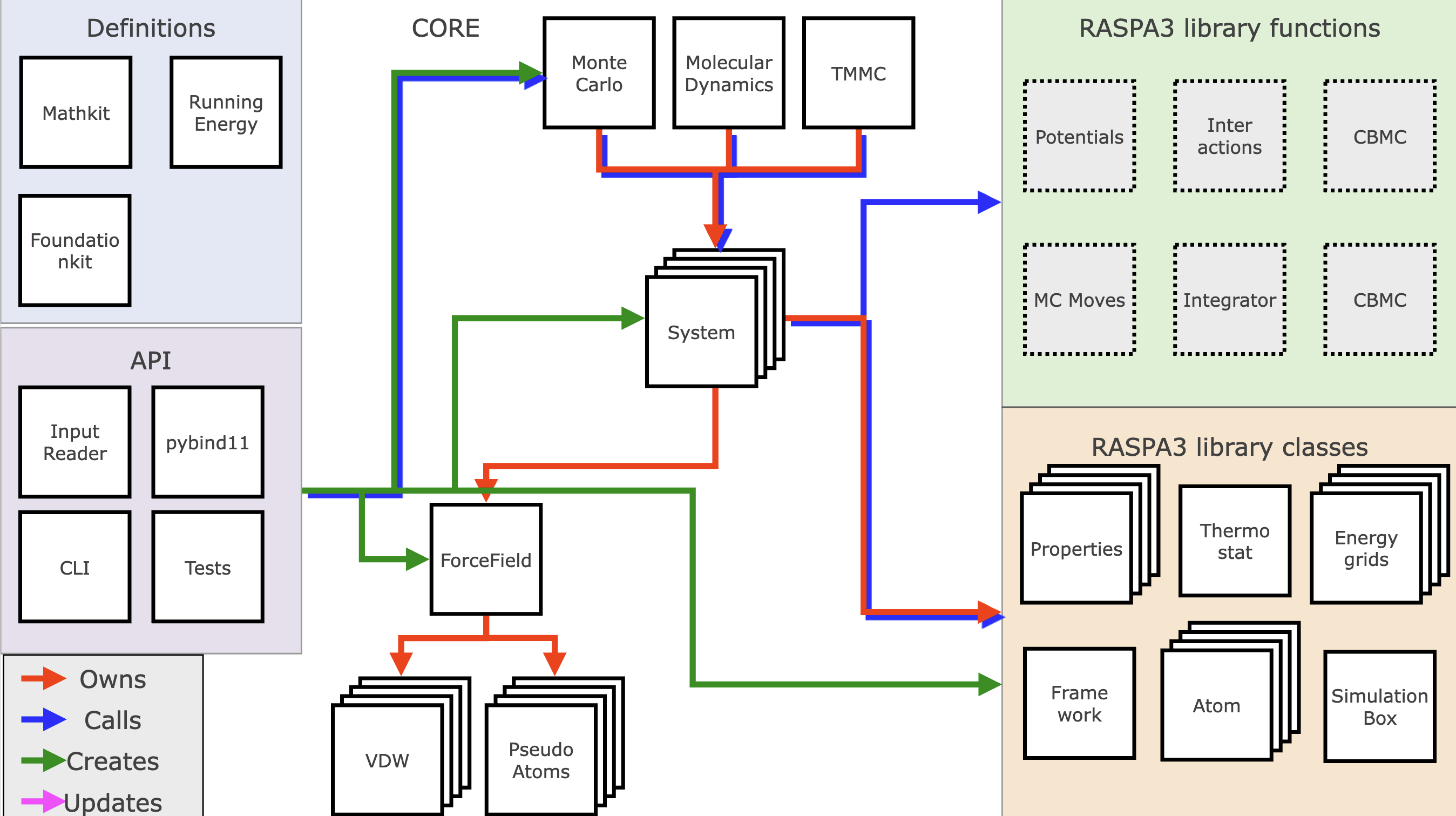
System structure

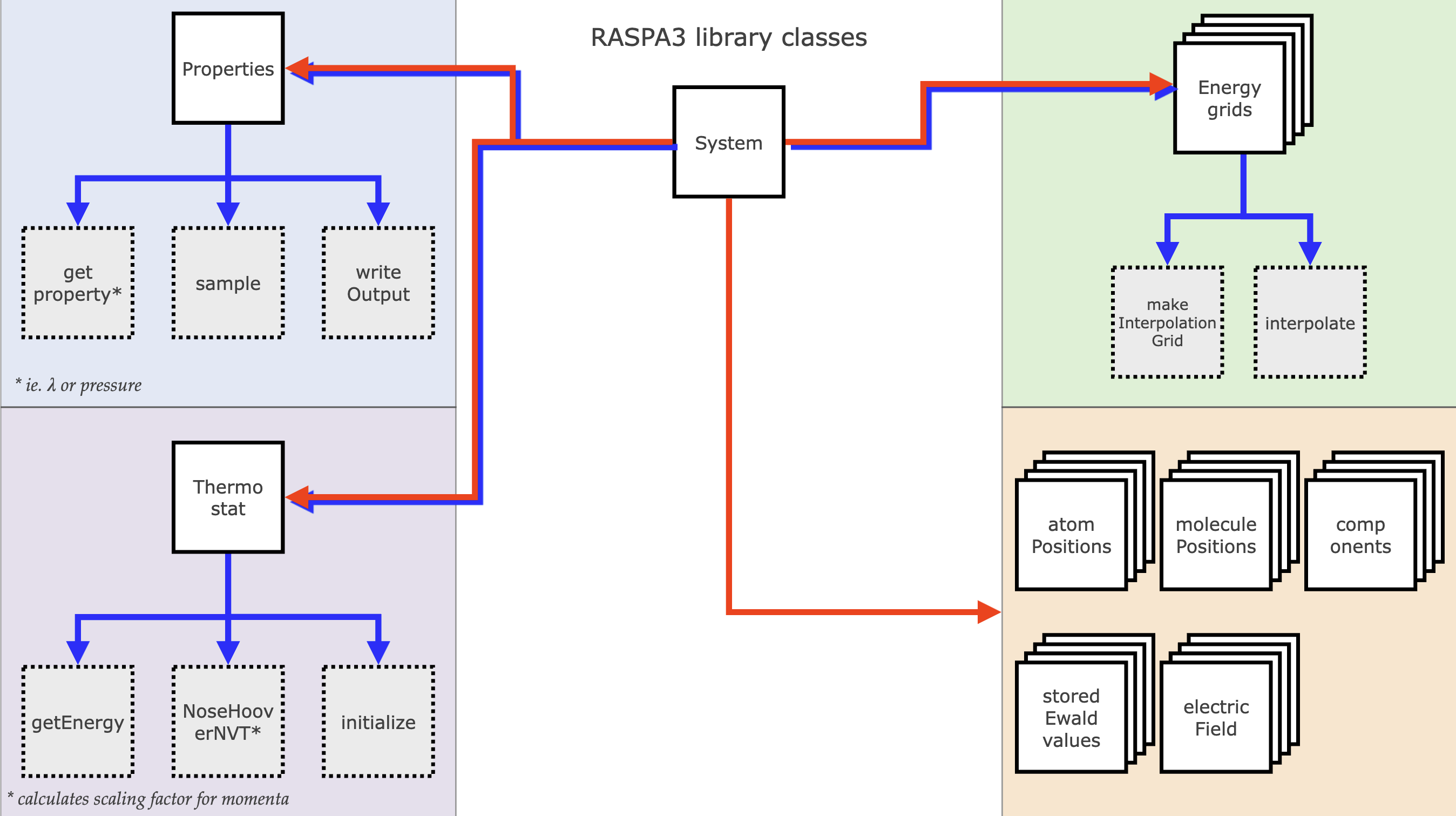
The System object is the main simulation object in is a container for all objects holding molecular information, property writers, the force field, the simulation box, framework and many others. Except for owning objects, some parts of RASPA are not object based, but are functions, routines that can operate on a given (reference to) set of data provided by the system. When function calls don't need data persistence between call, using a function is better.

The reason the system is the "owner" of all these objects is because they can vary between different systems, for example when using different force fields or simulation settings. The MonteCarlo object now starts the main simulation loop and operates on the system, by calling the various methods the system provides an interface to. For example, the MonteCarlo object can call a Monte Carlo move on the system, which will then propose and possibly accept a new state, which then updates the system state by updating its information.

MC Moves and MD Integrators

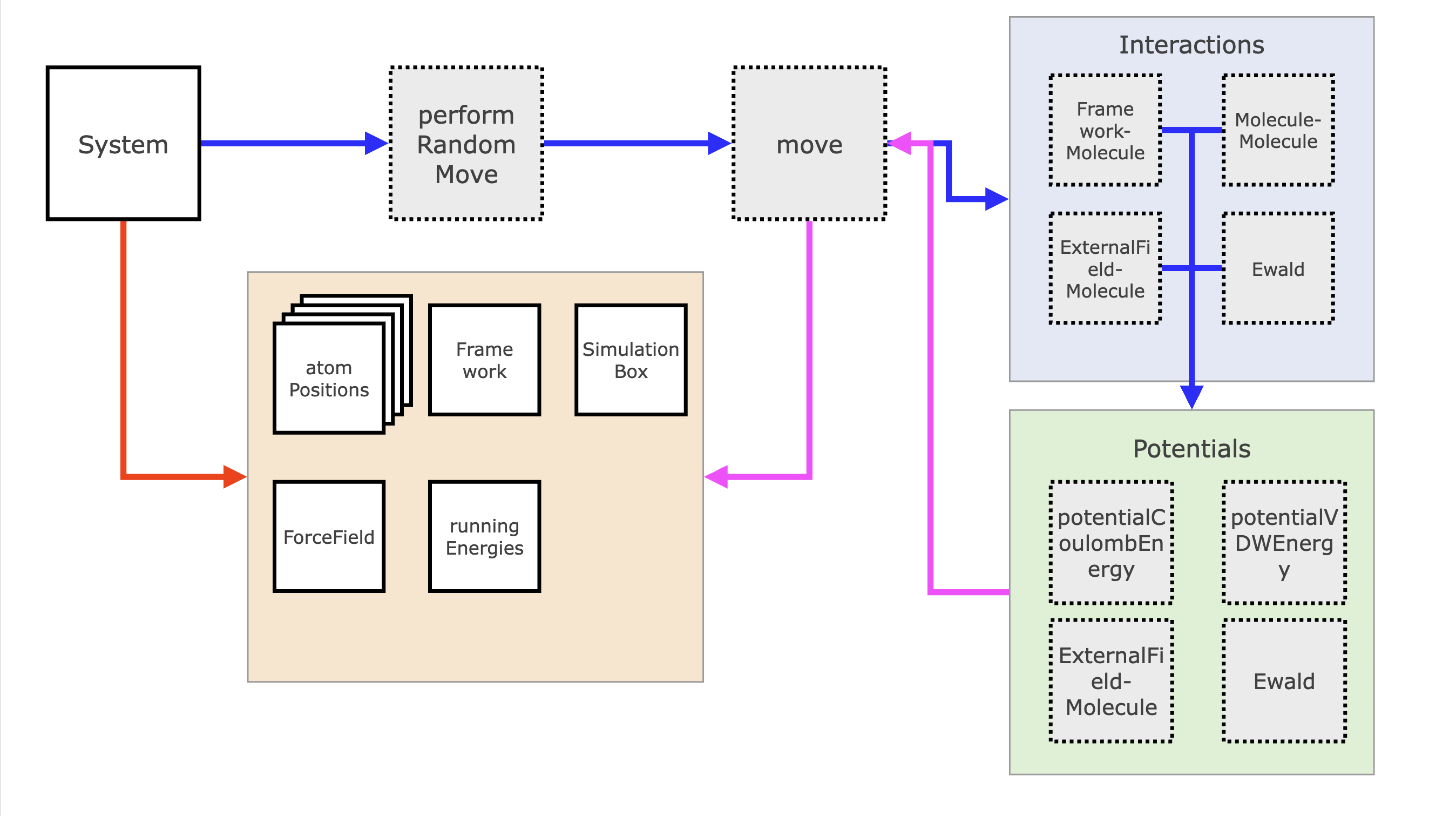
The general structure of a call to an MC move or to an MD integrator is actually quite similar. The System gets a call from the simulation routine to perform either a Monte Carlo move or MD integration step.

For the Monte Carlo move, it will first call performRandomMove, which will, based on the given probabilities per move, pick a random move. This move proposes a new state and calls Interactions routines, which calculate the energy difference. The Interactions routine splits up the energy into the different summed parts (internal, framework-molecule, molecule-molecule, etc.) and those routines loop over the relevant subselections of atoms and call Potentials. Potentials are functions that calculate the actual energy based on a distance and a set of parameters, such as the Lennard-Jones energy. As soon as this calculation has finished, the Monte Carlo move now calculates the transition probability between states and then will randomly either accept or reject the new state with the right probability. If the state is accepted the atomPositions and / or simulationBox are updated and the energy difference is returned and added to the energy accounting object runningEnergies.

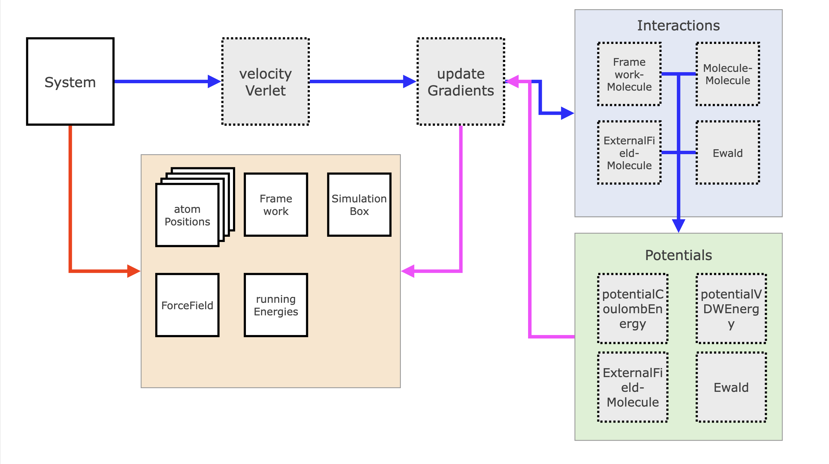
Similarly the System can call an integrator, for example velocityVerlet, which will then use the Velocity Verlet algorithm to calculate the half-step differences in the velocities and positions. Importantly, the gradients are updated using a function updateGradients, which will similarly use Interactions, which call Potentials to now calculate the energy and gradient of the different potential energy functions. velocityVerlet updates the positions and momenta again and optionally calls the thermostat to update the momenta again.

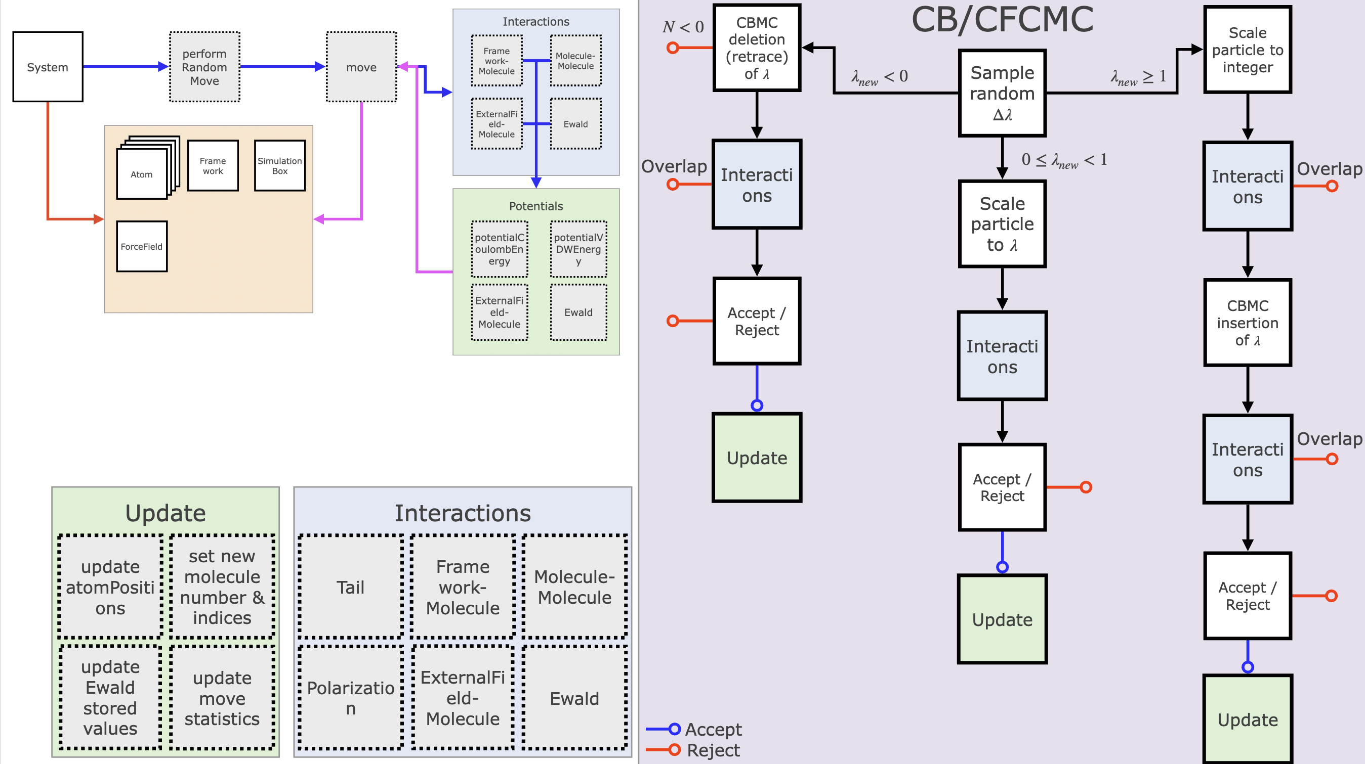
Example: CB/CFCMC Move

One example of a Monte Carlo move - which may also be the most complex move RASPA offers, is the "Configurational Bias Continuous Fractional Component Monte Carlo" move (our naming is still better than the DFT people name their XC functionals). The CB/CFCMC move is a combination of the CBMC move and the CFCMC move. The CBMC move increases the acceptance probability - and therefore decorrelation of the simulation - by proposing multiple possible states and selecting the best from the Boltzmann weight of the state with some extra accounting to keep detailed balance. CFCMC increases the acceptance by making one particle a fractional particle ($0 < \lambda <= 1$), such that the energy barrier of insertion is lower and more gradual.

The CB/CFCMC move starts by randomly sampling a random displacement $\Delta \lambda$, which alters the particle size. If $\lambda + \Delta \lamda < 1$ a deletion move is done (left branch in figure), else if $\lambda + \Delta \lamda \ge 1$ an insertion move is done, otherwise there will be just a scaling. If there is an insertion (deletion) taking place a new fractional particle should be placed (chosen), such that there is always 1 fractional particle. For this the CBMC routines are used. In all cases the new interaction energies are calculated and are then used to determine what the probability of acceptance of this move is. If this move is accepted, a set of routines is called (labeled Update in the figure) to alter the system state.