Table of Contents
- Monte Carlo: methane in box
- Monte Carlo: CO₂ and N₂ in two independent boxes
- Monte Carlo: binary mixture CO₂ and N₂ in box
- Monte Carlo: binary mixture propane and butane in box
- Molecular Dynamics: methane in box (msd)
- Monte Carlo: enthalpy of adsorption in MFI at zero loading
- Monte Carlo: Henry coefficient of methane in MFI
- Monte Carlo: adsorption of methane in MFI
- Monte Carlo: adsorption of butane in MFI
- Monte Carlo: adsorption of CO₂ in MFI
- Monte Carlo: adsorption of CO₂ in Cu-BTC
- Monte Carlo: Henry coefficient of methane, CO₂ and N₂ in MFI
- Monte Carlo: radial distribution function of water
- Molecular Dynamics: radial distribution function of water
Monte Carlo: methane in box
A Monte Carlo run of 100 methane molecules in a \(30 \times 30 \times 30\) Å box at 300K. After 1000 cycles of initialization the production run is started. A movie is written and every 10th configuration is appended to the movie. The movie is stored in ‘movies/’, and can be viewed with iRASPA or VMD.
The inputs for the simulation are specified in a json-file called simulation.json:
{
"SimulationType" : "MonteCarlo",
"NumberOfCycles" : 10000,
"NumberOfInitializationCycles" : 1000,
"PrintEvery" : 1000,
"Systems" :
[
{
"Type" : "Box",
"BoxLengths" : [30.0, 30.0, 30.0],
"ExternalTemperature" : 300.0,
"ChargeMethod" : "None",
"OutputPDBMovie" : true,
"SampleMovieEvery" : 10
}
],
"Components" :
[
{
"Name" : "methane",
"MoleculeDefinition" : "ExampleDefinitions",
"TranslationProbability" : 1.0,
"CreateNumberOfMolecules" : 100
}
]
}
There are global settings, but also settings for Systems and Components. The latter are arrays of sections with options. In this example, we specify one system of type Box with box-lengths \(30 \times 30 \times 30\) Å. We also set the option to make movies to true and sample the movie-snapshots every 10 cycles.
In RASPA, the cycle is define as max(20, \(N\)) steps, where \(N\) is the number of molecules in the system. In every cycle, each of the molecules has on average been used for a Monte Carlo move (accepted or rejected). There is a minimum of 20 steps to avoid that low-density systems or not sampled well. The definition of a cycle is less dependent on the system size. The number of Monte Carlo steps is roughly the number of cycles times the average number of molecules.
The forcefield is defined in force_field.json
{
"MixingRule" : "Lorentz-Berthelot",
"TruncationMethod" : "shifted",
"TailCorrections" : false,
"CutOffVDW" : 12.0,
"PseudoAtoms" :
[
{
"name" : "CH4",
"framework": false,
"print_to_output" : true,
"element" : "C",
"print_as" : "C",
"mass" : 16.04246,
"charge" : 0.0,
"source" : "M. G. Martin et al., J. Chem. Phys. 2001, 114, 7174-7181"
}
],
"SelfInteractions" :
[
{
"name" : "CH4",
"type" : "lennard-jones",
"parameters" : [158.5, 3.72],
"source" : "M. G. Martin et al., J. Chem. Phys. 2001, 114, 7174-7181."
}
]
}
where we defined the types of the atoms, and their parameters. Here we give them as self-interactions and a mixing rule. We use a cutoff of 12 Å shifted to zero at the cutoff, and omit tail-corrections.
The methane molecule is defined in methane.json
{
"CriticalTemperature" : 190.564,
"CriticalPressure" : 4599200.0,
"AcentricFactor" : 0.01142,
"Type" : "rigid",
"pseudoAtoms" :
[
["CH4",[0.0, 0.0, 0.0]]
]
}
which list the critical temperatures and acentric factors, used to convert pressure into fugacity for adsorption simulations, and the types of the atoms, along with their relative positions.
The output is written to the 'output' directory (one file per system), and the temperature and pressure are appended to all output filenames. In the output file, the simulation writes an important check to the file
Energy statistics | Energy [K] | Recomputed [K] | Drift [K] |
=============================================================================
Total potential energy | -1.892240e+04 | -1.892240e+04 | 3.412879e-10 |
molecule-molecule VDW | -1.892240e+04 | -1.892240e+04 | 3.412879e-10 |
-----------------------------------------------------------------------------
In Monte Carlo, only difference in energies are computed. These differences are continuously added to keep track of the current energies (from which average energies etc. are computed). Obviously, the current energy that is kept track off during the simulation should be equal to a full recalculation of the energies. The difference between the two signals an error. If the drift is higher than say \(10^{-3}\) or \(10^{-4}\) the results of the simulation are in error. This could be due to an error in one of the Monte Carlo moves or because the force field is `‘wrong’' (a typical error is when one forgets to define required potentials).
The performance of Monte Carlo moves is monitored. Translation moves are usually scaled to achieve an acceptance rate of 50%. Here, the move reached its upper limit of 1.5 Å because of the low density of the system.
Component 0 [methane]
Translation all: 1000000
Translation total: 333611 334052 332337
Translation constructed: 333340 333852 332065
Translation accepted: 265415 266313 264230
Translation fraction: 0.795582 0.797220 0.795066
Translation max-change: 1.500000 1.500000 1.500000
The last 3 columns correspond to the \(x\), \(y\), and \(z\) directions, respectively.
Averages are computed along with an error bar. The error is computed by dividing the simulation in 5 blocks and calculating the standard deviation. The errors in RASPA are computed as the 95% confidence interval.
Total energy:
-------------------------------------------------------------------------------
Block[ 0] -1.821186e+04
Block[ 1] -1.813742e+04
Block[ 2] -1.829147e+04
Block[ 3] -1.836916e+04
Block[ 4] -1.833114e+04
---------------------------------------------------------------------------
Average -1.826821e+04 +/- 1.160851e+02 [K]
Monte Carlo: CO₂ and N₂ in two independent boxes
RASPA has a build-in structure of being able to simulate several systems at the same time. This has applications in Gibbs-ensembles and (hyper) parallel tempering for example. However, this capability can also be used for independent systems. The first box is \(25 \times 25 \times 25\) Å with 90 \(^\circ\) angles, containing 100 N₂ and 0 CO₂ and molecules and moved around by translation, rotation and reinsertion. The second box is monoclinic and of size \(30 \times 30 \times 30\) with \(\beta = 120^\circ, \alpha = \gamma = 90^\circ\) containing 0 N₂ and 100 CO₂ molecules. The first system is at 300K, the second at 500K.
{
"SimulationType" : "MonteCarlo",
"NumberOfCycles" : 10000,
"NumberOfInitializationCycles" : 1000,
"PrintEvery" : 1000,
"Systems" :
[
{
"Type" : "Box",
"BoxLengths" : [25.0, 25.0, 25.0],
"ExternalTemperature" : 300.0,
"ChargeMethod" : "Ewald",
"OutputPDBMovie" : true,
"SampleMovieEvery" : 10
},
{
"Type" : "Box",
"BoxLengths" : [30.0, 30.0, 30.0],
"BoxAngles" : [90.0, 120.0, 90.0],
"ExternalTemperature" : 500.0,
"ChargeMethod" : "Ewald",
"OutputPDBMovie" : true,
"SampleMovieEvery" : 10
}
],
"Components" :
[
{
"Name" : "CO2",
"MoleculeDefinition" : "ExampleDefinitions",
"TranslationProbability" : 1.0,
"RotationProbability" : 1.0,
"ReinsertionProbability" : 1.0,
"CreateNumberOfMolecules" : [100, 0]
},
{
"Name" : "N2",
"MoleculeDefinition" : "ExampleDefinitions",
"TranslationProbability" : 1.0,
"RotationProbability" : 1.0,
"ReinsertionProbability" : 1.0,
"CreateNumberOfMolecules" : [0, 100]
}
]
}
with the N₂ defined as
{
"CriticalTemperature": 126.192,
"CriticalPressure": 3395800.0,
"AcentricFactor": 0.0372,
"Type": "rigid",
"pseudoAtoms": [
["N_n2", [0.0, 0.0, 0.55]],
["N_com", [0.0, 0.0, 0.0]],
["N_n2", [0.0, 0.0, -0.55]]
]
}
and CO₂ defined as
{
"CriticalTemperature": 304.1282,
"CriticalPressure": 7377300.0,
"AcentricFactor": 0.22394,
"Type": "rigid",
"pseudoAtoms": [
["O_co2", [0.0, 0.0, 1.149]],
["C_co2", [0.0, 0.0, 0.0]],
["O_co2", [0.0, 0.0, -1.149]]
]
}
The force field is defined as
{
"MixingRule" : "Lorentz-Berthelot",
"TruncationMethod" : "shifted",
"TailCorrections" : false,
"CutOffVDW" : 12.0,
"CutOffCoulomb" : "auto",
"PseudoAtoms" :
[
{
"name" : "C_co2",
"framework" : false,
"print_to_output" : true,
"element" : "C",
"print_as" : "C",
"mass" : 12.0,
"charge" : 0.6512,
"source" : "A. Garcia-Sanchez et al., J. Phys. Chem. C 2009, 113, 8814-8820"
},
{
"name" : "O_co2",
"framework" : false,
"print_to_output" : true,
"element" : "O",
"print_as" : "O",
"mass" : 15.9994,
"charge" : -0.3256,
"source" : "A. Garcia-Sanchez et al., J. Phys. Chem. C 2009, 113, 8814-8820"
},
{
"name" : "N_n2",
"framework" : false,
"print_to_output" : true,
"element" : "N",
"print_as" : "N",
"mass" : 14.00674,
"charge" : -0.405,
"source" : "A. Martin-Calvo et al. , Phys. Chem. Chem. Phys. 2011, 13, 11165-11174"
},
{
"name" : "N_com",
"framework" : false,
"print_to_output" : false,
"element" : "N",
"print_as" : "-",
"mass" : 0.0,
"charge" : 0.810,
"source" : "A. Martin-Calvo et al. , Phys. Chem. Chem. Phys. 2011, 13, 11165-11174"
}
],
"SelfInteractions" :
[
{
"name" : "O_co2",
"type" : "lennard-jones",
"parameters" : [85.671, 3.017],
"source" : "A. Garcia-Sanchez et al., J. Phys. Chem. C 2009, 113, 8814-8820"
},
{
"name" : "C_co2",
"type" : "lennard-jones",
"parameters" : [29.933, 2.745],
"source" : "A. Garcia-Sanchez et al., J. Phys. Chem. C 2009, 113, 8814-8820"
},
{
"name" : "N_n2",
"type" : "lennard-jones",
"parameters" : [38.298, 3.306],
"source" : "A. Martin-Calvo et al. , Phys. Chem. Chem. Phys. 2011, 13, 11165-11174"
},
{
"name" : "N_com",
"type" : "none",
"parameters" : [0.0, 1.0],
"source" : "A. Martin-Calvo et al. , Phys. Chem. Chem. Phys. 2011, 13, 11165-11174"
}
]
}
The CO₂ has the charges distrubted over the atoms to approximate the experimental quadrupole. For N₂ we can not do the same. However, we can add a "dummy" site in the center of the two nitrogen atoms to mimick the quadrupole. This N_com is placed at the center of mass and has no VDW interactions, and only acts as a charge-center.
Based on the self-interactions and the mixing rule, the cross-interactions are computed:
C_co2 - C_co2 Lennard-Jones p₀/kʙ: 29.93300 [K], p₁: 2.74500 [Å]
shift: -0.01715 [K], tailcorrections: false
C_co2 - O_co2 Lennard-Jones p₀/kʙ: 50.63981 [K], p₁: 2.88100 [Å]
shift: -0.03878 [K], tailcorrections: false
C_co2 - N_n2 Lennard-Jones p₀/kʙ: 33.85815 [K], p₁: 3.02550 [Å]
shift: -0.03478 [K], tailcorrections: false
C_co2 - N_com Lennard-Jones p₀/kʙ: 0.00000 [K], p₁: 1.87250 [Å]
shift: 0.00000 [K], tailcorrections: false
O_co2 - O_co2 Lennard-Jones p₀/kʙ: 85.67100 [K], p₁: 3.01700 [Å]
shift: -0.08653 [K], tailcorrections: false
O_co2 - N_n2 Lennard-Jones p₀/kʙ: 57.28026 [K], p₁: 3.16150 [Å]
shift: -0.07659 [K], tailcorrections: false
O_co2 - N_com Lennard-Jones p₀/kʙ: 0.00000 [K], p₁: 2.00850 [Å]
shift: 0.00000 [K], tailcorrections: false
N_n2 - N_n2 Lennard-Jones p₀/kʙ: 38.29800 [K], p₁: 3.30600 [Å]
shift: -0.06695 [K], tailcorrections: false
N_n2 - N_com Lennard-Jones p₀/kʙ: 0.00000 [K], p₁: 2.15300 [Å]
shift: 0.00000 [K], tailcorrections: false
N_com - N_com Lennard-Jones p₀/kʙ: 0.00000 [K], p₁: 1.00000 [Å]
shift: 0.00000 [K], tailcorrections: false
There will be an output-file for each system
output/output_300_0.s0.txt
output/output_500_0.s1.txt
Note that we specify only relative probabilities of MC particle moves. They will be correctly rescaled as shown in the output-file:
Translation-move probability: 0.3333333333333333 [-]
Rotation-move probability: 0.3333333333333333 [-]
Reinsertion (CBMC) probability: 0.3333333333333333 [-]
At every MC-step, each move will be randomly selected with 1/3 probability.
Monte Carlo: binary mixture CO₂ and N₂ in box
{
"SimulationType" : "MonteCarlo",
"NumberOfCycles" : 10000,
"NumberOfInitializationCycles" : 1000,
"PrintEvery" : 1000,
"Systems" :
[
{
"Type" : "Box",
"BoxLengths" : [25.0, 25.0, 25.0],
"ExternalTemperature" : 300.0,
"ChargeMethod" : "Ewald"
},
{
"Type" : "Box",
"BoxLengths" : [30.0, 30.0, 30.0],
"ExternalTemperature" : 500.0,
"ChargeMethod" : "Ewald"
}
],
"Components" :
[
{
"Name" : "CO2",
"MoleculeDefinition" : "ExampleDefinitions",
"TranslationProbability" : 1.0,
"RotationProbability" : 1.0,
"ReinsertionProbability" : 1.0,
"CreateNumberOfMolecules" : [50, 25]
},
{
"Name" : "N2",
"MoleculeDefinition" : "ExampleDefinitions",
"TranslationProbability" : 1.0,
"RotationProbability" : 1.0,
"ReinsertionProbability" : 1.0,
"CreateNumberOfMolecules" : [25, 50]
}
]
}
Monte Carlo: binary mixture propane and butane in box
A Monte Carlo run of 50 propane and 50 butane molecules in a \(30\times30\times30\) Å box. The MC moves are translation, rotation, full reinsertion, and partial reinsertion. After 1000 steps of initialization the production run is started. We run for 20,000 cycles to get some decent statistics.
{
"SimulationType" : "MonteCarlo",
"NumberOfCycles" : 20000,
"NumberOfInitializationCycles" : 5000,
"PrintEvery" : 1000,
"Systems" :
[
{
"Type" : "Box",
"BoxLengths" : [30.0, 30.0, 30.0],
"ExternalTemperature" : 500.0,
"ChargeMethod" : "None"
}
],
"Components" :
[
{
"Name" : "propane",
"TranslationProbability" : 1.0,
"RotationProbability" : 1.0,
"ReinsertionProbability" : 1.0,
"PartialReinsertionProbability" : 1.0,
"CreateNumberOfMolecules" : 50
},
{
"Name" : "butane",
"TranslationProbability" : 1.0,
"RotationProbability" : 1.0,
"ReinsertionProbability" : 1.0,
"PartialReinsertionProbability" : 1.0,
"CreateNumberOfMolecules" : 50
}
]
}
The propane and butane molecules are modeled as flexible united-atom beads. The intra-molecular force field contains bond and bend terms for propane.json
{
"CriticalTemperature" : 369.825,
"CriticalPressure" : 4247660.0,
"AcentricFactor" : 0.1524,
"Type" : "flexible",
"pseudoAtoms" :
[
["CH3", [0.0, 0.0, 0.0]],
["CH2", [0.0, 0.0, 0.0]],
["CH3", [0.0, 0.0, 0.0]]
],
"Connectivity" : [
[0, 1],
[1, 2]
],
"Bonds" : [
[["CH3", "CH2"], "FIXED", [1.54]]
],
"Bends" : [
[["CH3", "CH2", "CH3"], "HARMONIC", [62500.0, 114]]
],
"Partial-reinsertion" : [
[0, 1],
[1, 2],
[0],
[2]
]
}
and bond, bend, and torsion terms for butane.json
{
"CriticalTemperature" : 425.125,
"CriticalPressure" : 3796000.0,
"AcentricFactor" : 0.201,
"Type" : "flexible",
"pseudoAtoms" :
[
["CH3", [0.0, 0.0, 0.0]],
["CH2", [0.0, 0.0, 0.0]],
["CH2", [0.0, 0.0, 0.0]],
["CH3", [0.0, 0.0, 0.0]]
],
"Connectivity" : [
[0, 1],
[1, 2],
[2, 3]
],
"Bonds" : [
[["CH3", "CH2"], "FIXED", [1.54]],
[["CH2", "CH2"], "FIXED", [1.54]]
],
"Bends" : [
[["CH3", "CH2", "CH2"], "HARMONIC", [62500.0, 114]]
],
"Torsions" : [
[["CH3", "CH2", "CH2", "CH3"], "TRAPPE", [0.0, 355.03, -68.19, 791.32]]
],
"Partial-reinsertion" : [
[0, 1],
[2, 3],
[0],
[3]
]
}
The TraPPE forcefield is defined as
{
"MixingRule" : "Lorentz-Berthelot",
"TruncationMethod" : "truncated",
"TailCorrections" : true,
"CutOff" : 12.0,
"PseudoAtoms" :
[
{
"name" : "CH3",
"framework" : false,
"print_to_output" : true,
"element" : "C",
"print_as" : "C",
"mass" : 15.04,
"charge" : 0.0,
"source" : "M. G. Martin and J. I. Siepmann, J. Phys. Chem. B 1998, 102(14), 2569–2577."
},
{
"name" : "CH2",
"framework" : false,
"print_to_output" : true,
"element" : "C",
"print_as" : "C",
"mass" : 14.03,
"charge" : 0.0,
"source" : "M. G. Martin and J. I. Siepmann, J. Phys. Chem. B 1998, 102(14), 2569–2577."
}
],
"SelfInteractions" :
[
{
"name" : "CH3",
"type" : "lennard-jones",
"parameters" : [98.0, 3.75],
"source" : "M. G. Martin and J. I. Siepmann, J. Phys. Chem. B 1998, 102(14), 2569–2577."
},
{
"name" : "CH2",
"type" : "lennard-jones",
"parameters" : [46.0, 3.95],
"source" : "M. G. Martin and J. I. Siepmann, J. Phys. Chem. B 1998, 102(14), 2569–2577."
}
]
}
Energy statistics | Energy [K] | Recomputed [K]| Drift [K] |
===============================================================================
Total potential energy/kʙ | -2.963848e+04 | -2.963848e+04 | -1.520919e-08 |
molecule-molecule VDW/kʙ | -8.633271e+04 | -8.633271e+04 | -8.505944e-09 |
Van der Waals (Tail)/kʙ | -5.017238e+03 | -5.017238e+03 | 0.000000e+00 |
bond/kʙ | 0.000000e+00 | 0.000000e+00 | 0.000000e+00 |
bend/kʙ | 3.391890e+04 | 3.391890e+04 | -7.468954e-09 |
torsion/kʙ | 2.779257e+04 | 2.779257e+04 | 7.657100e-10 |
-------------------------------------------------------------------------------
The translation and rotation moves leave the internal structure invariant.
Component 0 [propane]
Translation all: 500633
Translation total: 167364 167001 166268
Translation constructed: 167355 166992 166263
Translation accepted: 103946 104914 105966
Translation fraction: 0.621077 0.628224 0.637320
Translation max-change: 1.500000 1.500000 1.500000
Rotation all: 499525
Rotation total: 166142 166594 166789
Rotation constructed: 164548 165646 165967
Rotation accepted: 100422 109640 110938
Rotation fraction: 0.604435 0.658127 0.665140
Rotation max-change: 1.500000 1.500000 1.500000
Component 1 [butane]
Translation all: 500514
Translation total: 167059 166424 167031
Translation constructed: 167053 166417 167023
Translation accepted: 103464 97379 98048
Translation fraction: 0.619326 0.585126 0.587005
Translation max-change: 1.500000 1.500000 1.500000
Rotation all: 499580
Rotation total: 166131 166746 166703
Rotation constructed: 163313 164838 164828
Rotation accepted: 95163 102118 102226
Rotation fraction: 0.572819 0.612416 0.613222
Rotation max-change: 1.230832 1.160213 1.172102
The reinsertion-move regrows the molecule at a random position with a new internal structure.
Component 0 [propane]
Reinsertion (CBMC) all: 499698
Reinsertion (CBMC) total: 499698
Reinsertion (CBMC) constructed: 499642
Reinsertion (CBMC) accepted: 268113
Reinsertion (CBMC) fraction: 0.536550
Reinsertion (CBMC) max-change: 0.000000
Component 1 [butane]
Reinsertion (CBMC) all: 498890
Reinsertion (CBMC) total: 498890
Reinsertion (CBMC) constructed: 498706
Reinsertion (CBMC) accepted: 215229
Reinsertion (CBMC) fraction: 0.431416
Reinsertion (CBMC) max-change: 0.000000
The acceptance percentages are here high enough. But for dense systems, the insertion acceptance ratios become too small. In these cases, other moves (like partial-reinsertion or MC/MD hybrid moves) become essential to properly sample the internal structure of molecules.
Component 0 [propane]
Partial reinsertion (CBMC) all: 500700
Partial reinsertion (CBMC) total: 500700
Partial reinsertion (CBMC) constructed: 500700
Partial reinsertion (CBMC) accepted: 392298
Partial reinsertion (CBMC) fraction: 0.783499
Partial reinsertion (CBMC) max-change: 0.000000
Component 1 [butane]
Partial reinsertion (CBMC) all: 500460
Partial reinsertion (CBMC) total: 500460
Partial reinsertion (CBMC) constructed: 500436
Partial reinsertion (CBMC) accepted: 315821
Partial reinsertion (CBMC) fraction: 0.631061
Partial reinsertion (CBMC) max-change: 0.000000
The average energies of the internal potentials are computed as:
Bend energy/kʙ 0 [propane]
---------------------------------------------------------------------------
Block[ 0] 1.240826e+04
Block[ 1] 1.237668e+04
Block[ 2] 1.251196e+04
Block[ 3] 1.243697e+04
Block[ 4] 1.245964e+04
-----------------------------------------------------------------------
Average 1.243870e+04 +/- 6.385477e+01 [K]
Bend energy/kʙ 1 [butane]
---------------------------------------------------------------------------
Block[ 0] 2.468257e+04
Block[ 1] 2.482497e+04
Block[ 2] 2.495069e+04
Block[ 3] 2.489606e+04
Block[ 4] 2.459066e+04
-----------------------------------------------------------------------
Average 2.478899e+04 +/- 1.857683e+02 [K]
Torsion energy/kʙ 1 [butane]
---------------------------------------------------------------------------
Block[ 0] 2.492220e+04
Block[ 1] 2.463722e+04
Block[ 2] 2.505684e+04
Block[ 3] 2.487121e+04
Block[ 4] 2.463080e+04
-----------------------------------------------------------------------
Average 2.482365e+04 +/- 2.308448e+02 [K]
In addition to the average energies, we also get information on the pressure:
Average pressure tensor:
-------------------------------------------------------------------------------
1.7178e+02 4.2992e-02 -1.2965e-03 +/- 1.1175e+01 4.4986e+00 2.0788e+00 [bar]
4.2992e-02 1.7332e+02 -2.1953e+00 +/- 4.4986e+00 5.9796e+00 3.6461e+00 [bar]
-1.2965e-03 -2.1953e+00 1.7461e+02 +/- 2.0788e+00 3.6461e+00 5.2866e+00 [bar]
Block[ 0] 2.556760e+07
Block[ 1] 2.556760e+07
Block[ 2] 2.556760e+07
Block[ 3] 2.556760e+07
Block[ 4] 2.556760e+07
---------------------------------------------------------------------------
Ideal gas pressure 2.556760e+07 +/- 0.000000e+00 [Pa]
2.556760e+02 +/- 0.000000e+00 [bar]
Block[ 0] -8.290629e+06
Block[ 1] -8.220314e+06
Block[ 2] -8.465780e+06
Block[ 3] -8.732872e+06
Block[ 4] -7.510238e+06
---------------------------------------------------------------------------
Excess pressure -8.243966e+06 +/- 5.652840e+05 [Pa]
-8.243966e+01 +/- 5.652840e+00 [bar]
Block[ 0] 1.727697e+07
Block[ 1] 1.734729e+07
Block[ 2] 1.710182e+07
Block[ 3] 1.683473e+07
Block[ 4] 1.805736e+07
---------------------------------------------------------------------------
Pressure average 1.732363e+07 +/- 5.652840e+05 [Pa]
1.732363e+02 +/- 5.652840e+00 [bar]
Molecular Dynamics: methane in box (msd)
A molecular dynamics run of a methane fluid at 300K and a density of 98.7 kg / m3. As no TimeStep is specified in the simulation.json the default value of timeStep = 5e-4 is used. We measure the MSD by setting ComputeMSD to true
{
"SimulationType" : "MolecularDynamics",
"NumberOfCycles" : 1000000,
"NumberOfInitializationCycles" : 1000,
"NumberOfEquilibrationCycles" : 10000,
"PrintEvery" : 10000,
"Systems" :
[
{
"Type" : "Box",
"BoxLengths" : [30.0, 30.0, 30.0],
"ExternalTemperature" : 300.0,
"ChargeMethod" : "None",
"Ensemble" : "NVT",
"ComputeMSD" : true,
"SampleMSDEvery" : 10,
"WriteMSDEvery" : 5000
}
],
"Components" :
[
{
"Name" : "methane",
"TranslationProbability" : 0.5,
"ReinsertionProbability" : 0.5,
"CreateNumberOfMolecules" : 100
}
]
}
We measure the average energies, which is just the Van der Waals contribution as methane is modelled as an uncharged, unpolarized point particle.
Energy averages and statistics:
===============================================================================
Inter-molecular energy contributions per energy type:
-------------------------------------------------------------------------------
Van der Waals energy/kʙ 0-0 [methane-methane]:
---------------------------------------------------------------------------
Block[ 0] -1.845790e+04
Block[ 1] -1.833565e+04
Block[ 2] -1.835129e+04
Block[ 3] -1.856717e+04
Block[ 4] -1.820499e+04
-----------------------------------------------------------------------
Average -1.838340e+04 +/- 1.693840e+02 [K]
...
Kinetic Energies:
-------------------------------------------------------------------------------
Translational Kinetic energy/kʙ
---------------------------------------------------------------------------
Block[ 0] 4.455050e+04
Block[ 1] 4.455015e+04
Block[ 2] 4.454971e+04
Block[ 3] 4.455030e+04
Block[ 4] 4.455015e+04
-----------------------------------------------------------------------
Average 4.455016e+04 +/- 3.642679e-01 [K]
Rotational Kinetic energy/kʙ
---------------------------------------------------------------------------
Block[ 0] 0.000000e+00
Block[ 1] 0.000000e+00
Block[ 2] 0.000000e+00
Block[ 3] 0.000000e+00
Block[ 4] 0.000000e+00
-----------------------------------------------------------------------
Average 0.000000e+00 +/- 0.000000e+00 [K]
Nose Hoover energy/kʙ
---------------------------------------------------------------------------
Block[ 0] -8.475074e+01
Block[ 1] -3.162406e+02
Block[ 2] -1.737929e+02
Block[ 3] -1.862179e+02
Block[ 4] -2.077868e+01
-----------------------------------------------------------------------
Average -1.563561e+02 +/- 1.391706e+02 [K]
...
Total energy/kʙ
-------------------------------------------------------------------------------
Block[ 0] -1.845790e+04
Block[ 1] -1.833565e+04
Block[ 2] -1.835129e+04
Block[ 3] -1.856717e+04
Block[ 4] -1.820499e+04
---------------------------------------------------------------------------
Average -1.838340e+04 +/- 1.693840e+02 [K]
And we measure the pressure
Pressure averages and statistics:
===============================================================================
Average pressure tensor:
-------------------------------------------------------------------------------
1.3030e+02 -9.7982e-02 5.0615e-01 +/- 1.0480e+00 9.4374e-01 6.2455e-01 [bar]
-9.7982e-02 1.2941e+02 -7.9968e-02 +/- 9.4374e-01 1.1444e+00 8.8396e-01 [bar]
5.0615e-01 -7.9968e-02 1.2939e+02 +/- 6.2455e-01 8.8396e-01 1.7600e+00 [bar]
Block[ 0] 1.534056e+07
Block[ 1] 1.534056e+07
Block[ 2] 1.534056e+07
Block[ 3] 1.534056e+07
Block[ 4] 1.534056e+07
---------------------------------------------------------------------------
Ideal gas pressure 1.534056e+07 +/- 0.000000e+00 [Pa]
1.534056e+02 +/- 0.000000e+00 [bar]
Block[ 0] -2.345817e+06
Block[ 1] -2.411870e+06
Block[ 2] -2.256290e+06
Block[ 3] -2.457657e+06
Block[ 4] -2.380705e+06
---------------------------------------------------------------------------
Excess pressure -2.370468e+06 +/- 9.427166e+04 [Pa]
-2.370468e+01 +/- 9.427166e-01 [bar]
Block[ 0] 1.299474e+07
Block[ 1] 1.292869e+07
Block[ 2] 1.308427e+07
Block[ 3] 1.288290e+07
Block[ 4] 1.295985e+07
---------------------------------------------------------------------------
Pressure average 1.297009e+07 +/- 9.427166e+04 [Pa]
1.297009e+02 +/- 9.427166e-01 [bar]
As we have also measured the MSD we can now plot the MSD over time and check the dynamics. We can see the ballistic regime, where the MSD scales with \(t^2\) and the diffusive regime where the MSD scales with \(t\).
import numpy as np
import matplotlib.pyplot as plt
import matplotlib as mpl
mpl.rcParams["font.size"] = 16
mpl.rcParams["figure.figsize"] = (8, 6)
msd = np.genfromtxt('msd/msd_self_methane.s0.txt')
fig, ax = plt.subplots()
ax.plot(msd[:, 0], msd[:, 1], label=r'$\langle | \mathbf{q}(t) - \mathbf{q}_0 |^2 \rangle$')
ax.plot(msd[:, 0], msd[:, 2], label=r'$\langle | x(t) - x_0 |^2 \rangle$')
ax.plot(msd[:, 0], msd[:, 3], label=r'$\langle | y(t) - y_0 |^2 \rangle$')
ax.plot(msd[:, 0], msd[:, 4], label=r'$\langle | z(t) - z_0 |^2 \rangle$')
x1 = np.logspace(0.5, 2.5, 5)
ax.plot(x1, 1e2 * x1, c='black', ls='--')
ax.annotate(r"$\sim D_0 t$", (1e1, 6e3))
x2 = np.logspace(-2.2, -0.2, 5)
ax.plot(x2, 1e2*x2**(2), c='black', ls='--')
ax.annotate(r"$\sim D_0 t^2$", (2e-2, 1e0))
ax.legend()
ax.set_xscale("log")
ax.set_yscale("log")
ax.set_xlabel(r"Time, $t$ / ps")
ax.set_ylabel(r"MSD / $\mathrm{\AA}^2$")
plt.savefig('example_basic_5_msd.png')

Monte Carlo: enthalpy of adsorption of methane in MFI at zero loading
{
"SimulationType" : "MonteCarlo",
"NumberOfCycles" : 5000,
"NumberOfInitializationCycles" : 5000,
"PrintEvery" : 1000,
"Systems" :
[
{
"Type" : "Framework",
"Name" : "MFI_SI",
"NumberOfUnitCells" : [2, 2, 2],
"HeliumVoidFraction" : 0.29,
"ExternalTemperature" : 300.0,
"ChargeMethod" : "None"
}
],
"Components" :
[
{
"Name" : "methane",
"MoleculeDefinition" : "ExampleDefinitions",
"TranslationProbability" : 0.5,
"ReinsertionProbability" : 0.5,
"CreateNumberOfMolecules" : 1
}
]
}
data_MFI
_cell_length_a 20.022
_cell_length_b 19.899
_cell_length_c 13.383
_cell_angle_alpha 90
_cell_angle_beta 90
_cell_angle_gamma 90
_cell_volume 5332.03
_symmetry_cell_setting orthorhombic
_symmetry_space_group_name_Hall '-P 2ac 2n'
_symmetry_space_group_name_H-M 'P n m a'
_symmetry_Int_Tables_number 62
loop_
_atom_site_label
_atom_site_type_symbol
_atom_site_fract_x
_atom_site_fract_y
_atom_site_fract_z
_atom_site_charge
Si Si 0.42238 0.0565 -0.33598 2.05
Si Si 0.30716 0.02772 -0.1893 2.05
Si Si 0.27911 0.06127 0.0312 2.05
Si Si 0.12215 0.06298 0.0267 2.05
Si Si 0.07128 0.02722 -0.18551 2.05
Si Si 0.18641 0.05896 -0.32818 2.05
Si Si 0.42265 -0.1725 -0.32718 2.05
Si Si 0.30778 -0.13016 -0.18548 2.05
Si Si 0.27554 -0.17279 0.03109 2.05
Si Si 0.12058 -0.1731 0.02979 2.05
Si Si 0.07044 -0.13037 -0.182 2.05
Si Si 0.18706 -0.17327 -0.31933 2.05
O O 0.3726 0.0534 -0.2442 -1.025
O O 0.3084 0.0587 -0.0789 -1.025
O O 0.2007 0.0592 0.0289 -1.025
O O 0.0969 0.0611 -0.0856 -1.025
O O 0.1149 0.0541 -0.2763 -1.025
O O 0.2435 0.0553 -0.246 -1.025
O O 0.3742 -0.1561 -0.2372 -1.025
O O 0.3085 -0.1552 -0.0728 -1.025
O O 0.198 -0.1554 0.0288 -1.025
O O 0.091 -0.1614 -0.0777 -1.025
O O 0.1169 -0.1578 -0.2694 -1.025
O O 0.2448 -0.1594 -0.2422 -1.025
O O 0.3047 -0.051 -0.1866 -1.025
O O 0.0768 -0.0519 -0.1769 -1.025
O O 0.4161 0.1276 -0.3896 -1.025
O O 0.4086 -0.0017 -0.4136 -1.025
O O 0.402 -0.1314 -0.4239 -1.025
O O 0.1886 0.1298 -0.3836 -1.025
O O 0.194 0.0007 -0.4082 -1.025
O O 0.1951 -0.1291 -0.419 -1.025
O O -0.0037 0.0502 -0.208 -1.025
O O -0.004 -0.1528 -0.2078 -1.025
O O 0.4192 -0.25 -0.354 -1.025
O O 0.1884 -0.25 -0.3538 -1.025
O O 0.2883 -0.25 0.0579 -1.025
O O 0.1085 -0.25 0.0611 -1.025
Total energy/kʙ
-------------------------------------------------------------------------------
Block[ 0] -1.986247e+03
Block[ 1] -1.983422e+03
Block[ 2] -1.985899e+03
Block[ 3] -1.984366e+03
Block[ 4] -1.984200e+03
---------------------------------------------------------------------------
Average -1.984827e+03 +/- 1.487712e+00 [K]
Monte Carlo: Henry coefficient of methane in MFI
{
"SimulationType" : "MonteCarlo",
"NumberOfCycles" : 20000,
"NumberOfInitializationCycles" : 0,
"PrintEvery" : 1000,
"ForceField" : ".",
"Systems" : [
{
"Type" : "Framework",
"Name" : "MFI_SI",
"NumberOfUnitCells" : [2, 2, 2],
"ExternalTemperature" : 300.0,
"ExternalPressure" : 1.0e5,
"ChargeMethod" : "None"
}
],
"Components" : [
{
"Name" : "methane",
"WidomProbability" : 1.0,
"IdealGasRosenbluthWeight" : 1.0,
"CreateNumberOfMolecules" : 0
}
]
}
Widom insertion Rosenbluth weight statistics:
---------------------------------------------------------------------------
Block[ 0] 2.732844e+01
Block[ 1] 2.741241e+01
Block[ 2] 2.736756e+01
Block[ 3] 2.745297e+01
Block[ 4] 2.738999e+01
---------------------------------------------------------------------------
Average Rosenbluth weight: 2.739027e+01 +/- 5.809780e-02 [-]
Henry coefficient based on Rosenbluth weight:
---------------------------------------------------------------------------
Block[ 0] 4.349384e-06
Block[ 1] 4.362748e-06
Block[ 2] 4.355610e-06
Block[ 3] 4.369203e-06
Block[ 4] 4.359181e-06
---------------------------------------------------------------------------
Average Henry coefficient: 4.359225e-06 +/- 9.246399e-09 [mol/kg/Pa]
Average Henry coefficient: 3.526013e-05 +/- 7.479065e-08 [molec./uc/Pa]
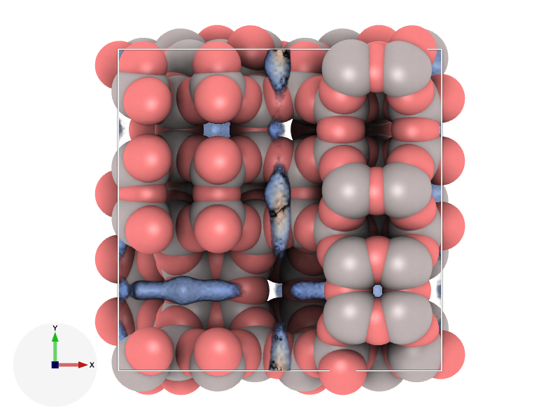
Monte Carlo: adsorption of methane in MFI
{
"SimulationType" : "MonteCarlo",
"NumberOfCycles" : 50000,
"NumberOfInitializationCycles" : 5000,
"PrintEvery" : 1000,
"Systems" : [
{
"Type" : "Framework",
"Name" : "MFI_SI",
"NumberOfUnitCells" : [2, 2, 2],
"ExternalTemperature" : 300.0,
"ExternalPressure" : 1.0e5,
"ChargeMethod" : "None",
"ComputeDensityGrid" : true,
"SampleDensityGridEvery" : 10,
"WriteDensityGridEvery" : 5000,
"DensityGridSize" : [128, 128, 128]
}
],
"Components" : [
{
"Name" : "methane",
"FugacityCoefficient" : 1.0,
"IdealGasRosenbluthWeight" : 1.0,
"TranslationProbability" : 0.5,
"ReinsertionProbability" : 0.5,
"SwapProbability" : 1.0,
"WidomProbability" : 1.0,
"CreateNuMberofmolecules" : 0
}
]
}
Component 0 (methane)
Block[ 0] 2.313265e+01
Block[ 1] 2.312087e+01
Block[ 2] 2.316992e+01
Block[ 3] 2.315223e+01
Block[ 4] 2.315949e+01
---------------------------------------------------------------------------
Abs. loading average 2.314703e+01 +/- 2.480976e-02 [molecules/cell]
Abs. loading average 2.893379e+00 +/- 3.101220e-03 [molecules/uc]
Abs. loading average 3.577097e-01 +/- 3.834051e-04 [mol/kg-framework]
Abs. loading average 5.738543e+00 +/- 6.150761e-03 [mg/g-framework]
Block[ 0] 2.210055e+01
Block[ 1] 2.208877e+01
Block[ 2] 2.213782e+01
Block[ 3] 2.212013e+01
Block[ 4] 2.212739e+01
---------------------------------------------------------------------------
Excess loading average 2.211493e+01 +/- 2.480976e-02 [molecules/cell]
Excess loading average 2.764367e+00 +/- 3.101220e-03 [molecules/uc]
Excess loading average 3.417598e-01 +/- 3.834051e-04 [mol/kg-framework]
Excess loading average 5.482668e+00 +/- 6.150761e-03 [mg/g-framework]
Component 0 [methane]
-------------------------------------------------------------------------------
Block[ 0] -2.315836e+03
Block[ 1] -2.318128e+03
Block[ 2] -2.316719e+03
Block[ 3] -2.316961e+03
Block[ 4] -2.318220e+03
---------------------------------------------------------------------------
Enthalpy of adsorption: -2.317173e+03 +/- 1.248718e+00 [K]
-1.926605e+01 +/- 1.038242e-02 [kJ/mol]
Warning: need to subtract the ideal-gas energy.
Component 0 [methane]
Reinsertion (CBMC) all: 19743492
Reinsertion (CBMC) total: 19743492
Reinsertion (CBMC) constructed: 16997136
Reinsertion (CBMC) accepted: 3589911
Reinsertion (CBMC) fraction: 0.181828
Reinsertion (CBMC) max-change: 0.000000
Translation all: 19749581
Translation total: 6581839 6587371 6580371
Translation constructed: 6581733 6587300 6580362
Translation accepted: 3767703 3755567 3293183
Translation fraction: 0.572439 0.570116 0.500456
Translation max-change: 1.500000 1.500000 1.337404
Swap (CBMC) all: 39481509
Swap (CBMC) total: 19743020 19738489 0
Swap (CBMC) constructed: 16955288 19738489 0
Swap (CBMC) accepted: 5907149 5907153 0
Swap (CBMC) fraction: 0.299202 0.299271 0.000000
Swap (CBMC) max-change: 0.000000 0.000000 0.000000
Widom insertion chemical potential statistics:
---------------------------------------------------------------------------
Block[ 0] -941.5351279073475
Block[ 1] -941.669377429965
Block[ 2] -941.2687442002162
Block[ 3] -941.1908992648339
Block[ 4] -941.1534302104509
---------------------------------------------------------------------------
Excess chemical potential: -9.413635e+02 +/- 2.816759e-01 [K]
Tail-correction chemical potential: 0.000000e+00 +/- 0.000000e+00 [K]
Ideal chemical potential: -2.255720e+03 +/- 3.215800e-01 [K]
Total chemical potential: -3.197084e+03 +/- 5.866208e-01 [K]
Imposed chemical potential: -3.189455e+03 [K]
---------------------------------------------------------------------------
Excess chemical potential: -7.826934e+00 +/- 2.341984e-03 [kJ/mol]
Tail-correction chemical potential: 0.000000e+00 +/- 0.000000e+00 [kj/mol]
Ideal chemical potential: -1.875511e+01 +/- 2.673766e-03 [kJ/mol]
Total chemical potential: -2.658204e+01 +/- 4.877438e-03 [kJ/mol]
Imposed chemical potential: -2.651861e+01 [kJ/mol]
---------------------------------------------------------------------------
Imposed fugacity: 1.000000e+05 [Pa]
Measured fugacity: 9.748910e+04 +/- 1.905630e+02 [Pa]
Monte Carlo: adsorption of butane in MFI
{
"SimulationType" : "MonteCarlo",
"NumberOfCycles" : 20000,
"NumberOfInitializationCycles" : 5000,
"PrintEvery" : 1000,
"Systems" : [
{
"Type" : "Framework",
"Name" : "MFI_SI",
"NumberOfUnitCells" : [2, 2, 2],
"ExternalTemperature" : 300.0,
"ExternalPressure" : 1.0e5,
"ChargeMethod" : "None"
}
],
"Components" : [
{
"Name" : "butane",
"FugacityCoefficient" : 1.0,
"IdealGasRosenbluthWeight" : 0.1304441,
"TranslationProbability" : 0.5,
"RotationProbability" : 0.5,
"ReinsertionProbability" : 0.5,
"SwapProbability" : 1.0,
"WidomProbability" : 1.0,
"CreateNumberOfMolecules" : 0
}
]
}
Component 0 (butane)
Block[ 0] 4.897422e+01
Block[ 1] 4.911684e+01
Block[ 2] 4.854518e+01
Block[ 3] 4.898799e+01
Block[ 4] 4.913708e+01
---------------------------------------------------------------------------
Abs. loading average 4.895226e+01 +/- 2.968620e-01 [molecules/cell]
Abs. loading average 6.119033e+00 +/- 3.710775e-02 [molecules/uc]
Abs. loading average 1.060962e+00 +/- 6.434008e-03 [mol/kg-framework]
Abs. loading average 6.171597e+01 +/- 3.742652e-01 [mg/g-framework]
Widom insertion chemical potential statistics:
---------------------------------------------------------------------------
Block[ 0] -3229.528393446422
Block[ 1] -3229.4951993384507
Block[ 2] -3237.13549982758
Block[ 3] -3230.6367434433205
Block[ 4] -3226.4629229725147
---------------------------------------------------------------------------
Excess chemical potential: -3.230658e+03 +/- 4.894948e+00 [K]
Tail-correction chemical potential: 0.000000e+00 +/- 0.000000e+00 [K]
Ideal chemical potential: -2.031027e+03 +/- 1.823937e+00 [K]
Total chemical potential: -5.261684e+03 +/- 6.668591e+00 [K]
Imposed chemical potential: -5.261783e+03 [K]
---------------------------------------------------------------------------
Excess chemical potential: -2.686119e+01 +/- 4.069887e-02 [kJ/mol]
Tail-correction chemical potential: 0.000000e+00 +/- 0.000000e+00 [kj/mol]
Ideal chemical potential: -1.688690e+01 +/- 1.516506e-02 [kJ/mol]
Total chemical potential: -4.374809e+01 +/- 5.544577e-02 [kJ/mol]
Imposed chemical potential: -4.374891e+01 [kJ/mol]
---------------------------------------------------------------------------
Imposed fugacity: 1.000000e+02 [Pa]
Measured fugacity: 1.000331e+02 +/- 2.205947e+00 [Pa]
Monte Carlo: adsorption of CO₂ in MFI
{
"SimulationType" : "MonteCarlo",
"NumberOfCycles" : 100000,
"NumberOfInitializationCycles" : 50000,
"NumberOfEquilibrationCycles" : 50000,
"PrintEvery" : 5000,
"Systems" :
[
{
"Type" : "Framework",
"Name" : "MFI_SI",
"HeliumVoidFraction" : 0.3,
"NumberOfUnitCells" : [2, 2, 2],
"ExternalTemperature" : 353.0,
"ExternalPressure" : 1.0e5,
"ChargeMethod" : "Ewald"
}
],
"Components" :
[
{
"Name" : "CO2",
"MoleculeDefinition" : "ExampleDefinitions",
"FugacityCoefficient" : 1.0,
"TranslationProbability" : 0.5,
"RotationProbability" : 0.5,
"ReinsertionProbability" : 0.5,
"SwapProbability" : 1.0,
"WidomProbability" : 1.0,
"CreateNumberOfMolecules" : 0
}
]
}
Component 0 (CO2)
Block[ 0] 2.601000e+01
Block[ 1] 2.651520e+01
Block[ 2] 2.645855e+01
Block[ 3] 2.631695e+01
Block[ 4] 2.613330e+01
---------------------------------------------------------------------------
Abs. loading average 2.628680e+01 +/- 2.653616e-01 [molecules/cell]
Abs. loading average 3.285850e+00 +/- 3.317020e-02 [molecules/uc]
Abs. loading average 4.062310e-01 +/- 4.100846e-03 [mol/kg-framework]
Abs. loading average 1.787368e+01 +/- 1.804323e-01 [mg/g-framework]
Block[ 0] 2.574659e+01
Block[ 1] 2.625179e+01
Block[ 2] 2.619514e+01
Block[ 3] 2.605354e+01
Block[ 4] 2.586989e+01
---------------------------------------------------------------------------
Excess loading average 2.602339e+01 +/- 2.653616e-01 [molecules/cell]
Excess loading average 3.252923e+00 +/- 3.317020e-02 [molecules/uc]
Excess loading average 4.021603e-01 +/- 4.100846e-03 [mol/kg-framework]
Excess loading average 1.769457e+01 +/- 1.804323e-01 [mg/g-framework]
Monte Carlo: adsorption of CO₂ in Cu-BTC
{
"SimulationType" : "MonteCarlo",
"NumberOfCycles" : 100000,
"NumberOfInitializationCycles" : 20000,
"PrintEvery" : 5000,
"Systems" : [
{
"Type" : "Framework",
"Name" : "Cu-BTC",
"NumberOfUnitCells" : [1, 1, 1],
"ChargeMethod" : "Ewald",
"ExternalTemperature" : 323.0,
"ExternalPressure" : 1.0e4
}
],
"Components" : [
{
"Name" : "CO2",
"FugacityCoefficient" : 1.0,
"IdealGasRosenbluthWeight" : 1.0,
"TranslationProbability" : 0.5,
"RotationProbability" : 0.5,
"ReinsertionProbability" : 0.5,
"SwapProbability" : 1.0,
"WidomProbability" : 1.0,
"CreateNumberOfMolecules" : 0
}
]
}
data_Cu-BTC
_cell_length_a 26.343
_cell_length_b 26.343
_cell_length_c 26.343
_cell_angle_alpha 90
_cell_angle_beta 90
_cell_angle_gamma 90
_cell_volume 18280.8
_symmetry_cell_setting cubic
_symmetry_space_group_name_Hall '-F 4 2 3'
_symmetry_space_group_name_H-M 'F m -3 m'
_symmetry_Int_Tables_number 225
loop_
_atom_site_label
_atom_site_type_symbol
_atom_site_fract_x
_atom_site_fract_y
_atom_site_fract_z
_atom_site_charge
Cu1 Cu 0.2853 0.2853 0 1.248
O1 O 0.3166 0.2431 0.9478 -0.624
C1 C 0.2968 0.2032 0.9313 0.494
C2 C 0.322 0.178 0.887 0.130
C3 C 0.3655 0.1994 0.8655 -0.156
H1 H 0.3802 0.228 0.8802 0.156
{
"MixingRule" : "Lorentz-Berthelot",
"TruncationMethod" : "shifted",
"TailCorrections" : false,
"CutOffVDW" : 12.0,
"PseudoAtoms" :
[
{
"name" : "Cu1",
"framework" : true,
"print_to_output" : true,
"element" : "Cu",
"print_as" : "Cu",
"mass" : 63.546039732,
"charge" : 1.248
},
{
"name" : "O1",
"framework" : true,
"print_to_output" : true,
"element" : "O",
"print_as" : "O",
"mass" : 15.999404927,
"charge" : -0.624
},
{
"name" : "C1",
"framework" : true,
"print_to_output" : true,
"element" : "C",
"print_as" : "C",
"mass" : 12.010735897,
"charge" : 0.494
},
{
"name" : "C2",
"framework" : true,
"print_to_output" : true,
"element" : "C",
"print_as" : "C",
"mass" : 12.010735897,
"charge" : 0.13
},
{
"name" : "C3",
"framework" : true,
"print_to_output" : true,
"element" : "C",
"print_as" : "C",
"mass" : 12.010735897,
"charge" : -0.156
},
{
"name" : "H1",
"framework" : true,
"print_to_output" : true,
"element" : "H",
"print_as" : "H",
"mass" : 1.007940754,
"charge" : 0.156
},
{
"name" : "C_co2",
"framework" : false,
"print_to_output" : true,
"element" : "C",
"print_as" : "C",
"mass" : 12.0,
"charge" : 0.6512
},
{
"name" : "O_co2",
"framework" : false,
"print_to_output" : true,
"element" : "O",
"print_as" : "O",
"mass" : 15.9994,
"charge" : -0.3256
}
],
"SelfInteractions" :
[
{
"name" : "Cu1",
"type" : "lennard-jones",
"parameters" : [2.5161, 3.11369],
"source" : "UFF"
},
{
"name" : "O1",
"type" : "lennard-jones",
"parameters" : [48.1581, 3.03315],
"source" : "DREIDING S.L. Mayo et al., J. Phys. Chem. 1990, 94, 8897-8909"
},
{
"name" : "C1",
"type" : "lennard-jones",
"parameters" : [47.8562, 3.47299],
"source" : "DREIDING S.L. Mayo et al., J. Phys. Chem. 1990, 94, 8897-8909"
},
{
"name" : "C2",
"type" : "lennard-jones",
"parameters" : [47.8562, 3.47299],
"source" : "DREIDING S.L. Mayo et al., J. Phys. Chem. 1990, 94, 8897-8909"
},
{
"name" : "C3",
"type" : "lennard-jones",
"parameters" : [47.8562, 3.47299],
"source" : "DREIDING S.L. Mayo et al., J. Phys. Chem. 1990, 94, 8897-8909"
},
{
"name" : "H1",
"type" : "lennard-jones",
"parameters" : [7.64893, 2.84642],
"source" : "DREIDING S.L. Mayo et al., J. Phys. Chem. 1990, 94, 8897-8909"
},
{
"name" : "O_co2",
"type" : "lennard-jones",
"parameters" : [85.671, 3.017],
"source" : "A. Garcia-Sanchez et al., J. Phys. Chem. C 2009, 113, 8814-8820"
},
{
"name" : "C_co2",
"type" : "lennard-jones",
"parameters" : [29.933, 2.745],
"source" : "A. Garcia-Sanchez et al., J. Phys. Chem. C 2009, 113, 8814-8820"
}
]
}
Monte Carlo: Henry coefficient of methane, CO₂ and N₂ in MFI
{
"SimulationType" : "MonteCarlo",
"NumberOfCycles" : 20000,
"NumberOfInitializationCycles" : 0,
"PrintEvery" : 1000,
"ForceField" : ".",
"Systems" : [
{
"Type" : "Framework",
"Name" : "MFI_SI",
"NumberOfUnitCells" : [2, 2, 2],
"ExternalTemperature" : 300.0,
"ExternalPressure" : 1.0e5,
"ChargeMethod" : "None"
}
],
"Components" : [
{
"Name" : "CO2",
"WidomProbability" : 1.0,
"CreateNumberOfMolecules" : 0
},
{
"Name" : "N2",
"WidomProbability" : 1.0,
"CreateNumberOfMolecules" : 0
},
{
"Name" : "methane",
"WidomProbability" : 1.0,
"CreateNumberOfMolecules" : 0
}
]
}
Monte Carlo: radial distribution function of water
{
"SimulationType" : "MolecularDynamics",
"NumberOfCycles" : 10000,
"NumberOfInitializationCycles" : 5000,
"NumberOfEquilibrationCycles" : 20000,
"PrintEvery" : 5000,
"Systems" :
[
{
"Type" : "Box",
"BoxLengths" : [24.83, 24.83, 24.83],
"ExternalTemperature" : 298.0,
"Ensemble" : "NVT",
"ChargeMethod" : "Ewald",
"OutputPDBMovie" : false,
"SampleMovieEvery" : 10,
"ComputeConventionalRDF" : true,
"NumberOfBinsConventionalRDF" : 128,
"RangeConventionalRDF" : 12.0,
"WriteConventionalRDFEvery" : 100
}
],
"Components" :
[
{
"Name" : "water",
"TranslationProbability" : 0.5,
"RotationProbability" : 0.5,
"ReinsertionProbability" : 1.0,
"CreateNumberOfMolecules" : 512
}
]
}
Molecular Dynamics: radial distribution function of water
{
"SimulationType" : "MonteCarlo",
"NumberOfCycles" : 10000,
"NumberOfInitializationCycles" : 10000,
"PrintEvery" : 100,
"Systems" :
[
{
"Type" : "Box",
"BoxLengths" : [24.83, 24.83, 24.83],
"ExternalTemperature" : 298.0,
"ChargeMethod" : "Ewald",
"OutputPDBMovie" : false,
"SampleMovieEvery" : 10,
"ComputeConventionalRDF" : true,
"NumberOfBinsConventionalRDF" : 128,
"RangeConventionalRDF" : 12.0,
"WriteConventionalRDFEvery" : 100
}
],
"Components" :
[
{
"Name" : "water",
"TranslationProbability" : 0.5,
"RotationProbability" : 0.5,
"ReinsertionProbability" : 1.0,
"CreateNumberOfMolecules" : 512
}
]
}